ESOL classification#
In this tutorial we provide a simple example of training a random forest classifier on the ESOL dataset,
a dataset of molecules and their aqueous solubility. We require the rdkit package, so make sure to pip install 'molflux[rdkit]' to follow along!
Loading the ESOL dataset#
First, let’s load the ESOL dataset
from molflux.datasets import load_dataset

dataset = load_dataset("esol")

print(dataset)

dataset[0]
Repo card metadata block was not found. Setting CardData to empty.
Dataset({
    features: ['smiles', 'log_solubility'],
    num_rows: 1126
})
{'smiles': 'OCC3OC(OCC2OC(OC(C#N)c1ccccc1)C(O)C(O)C2O)C(O)C(O)C3O ',
 'log_solubility': -0.77}
The loaded dataset is an instance of a HuggingFace Dataset (for more info, checkout the docs).
You can see that there are two columns: smiles and log_solubility. This is originally a regression dataset, but we’ll
threshold it at -3 to make it into a classification dataset
dataset = dataset.add_column(
    "log_solubility_cls",
    [0 if x < -3 else 1 for x in dataset["log_solubility"]]
)

print(dataset)
print(dataset[0])
Dataset({
    features: ['smiles', 'log_solubility', 'log_solubility_cls'],
    num_rows: 1126
})
{'smiles': 'OCC3OC(OCC2OC(OC(C#N)c1ccccc1)C(O)C(O)C2O)C(O)C(O)C3O ', 'log_solubility': -0.77, 'log_solubility_cls': 1}
As you can see, we now have a class column.
Featurising#
Now, we will featurise the dataset. For this, we will use the Morgan and MACCS fingerprints from rdkit and the
featurise_dataset function from molflux.datasets.
from molflux.datasets import featurise_dataset
from molflux.features import load_from_dicts as load_representations_from_dicts

featuriser = load_representations_from_dicts(
    [
        {"name": "morgan"},
        {"name": "maccs_rdkit"},
    ]
)

featurised_dataset = featurise_dataset(dataset, column="smiles", representations=featuriser)

print(featurised_dataset)
Dataset({
    features: ['smiles', 'log_solubility', 'log_solubility_cls', 'smiles::morgan', 'smiles::maccs_rdkit'],
    num_rows: 1126
})
You can see that we now have two extra columns for each fingerprint we used.
Splitting#
Next, we need to split the dataset. For this, we use the simple shuffle_split (random split) with 80% training and
20% test. To split the dataset, we use the split_dataset function from molflux.datasets.
from molflux.datasets import split_dataset
from molflux.splits import load_from_dict as load_split_from_dict

shuffle_strategy = load_split_from_dict(
    {
        "name": "shuffle_split",
        "presets": {
            "train_fraction": 0.8,
            "validation_fraction": 0.0,
            "test_fraction": 0.2,
        }
    }
)

split_featurised_dataset = next(split_dataset(featurised_dataset, shuffle_strategy))

print(split_featurised_dataset)
DatasetDict({
    train: Dataset({
        features: ['smiles', 'log_solubility', 'log_solubility_cls', 'smiles::morgan', 'smiles::maccs_rdkit'],
        num_rows: 900
    })
    validation: Dataset({
        features: ['smiles', 'log_solubility', 'log_solubility_cls', 'smiles::morgan', 'smiles::maccs_rdkit'],
        num_rows: 0
    })
    test: Dataset({
        features: ['smiles', 'log_solubility', 'log_solubility_cls', 'smiles::morgan', 'smiles::maccs_rdkit'],
        num_rows: 226
    })
})
Training the model#
We can now turn to training the model! We choose the random_forest_classifier (which we access from the sklearn package).
To do so, we need to define the model config and the x_features and the y_features.
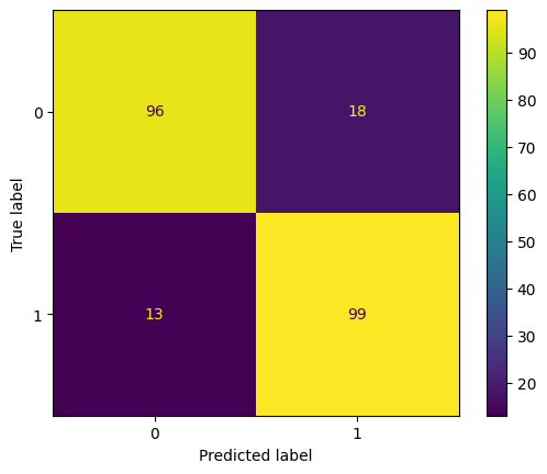
Once trained, we will get some predictions and compute some metrics and the confusion matrix!
import json

from molflux.modelzoo import load_from_dict as load_model_from_dict
from molflux.metrics import load_suite

from sklearn.metrics import confusion_matrix, ConfusionMatrixDisplay

import matplotlib.pyplot as plt

model = load_model_from_dict(
    {
        "name": "random_forest_classifier",
        "config": {
            "x_features": ['smiles::morgan', 'smiles::maccs_rdkit'],
            "y_features": ['log_solubility_cls'],
        }
    }
)

model.train(split_featurised_dataset["train"])

preds = model.predict(split_featurised_dataset["test"])

regression_suite = load_suite("classification")

scores = regression_suite.compute(
    references=split_featurised_dataset["test"]["log_solubility_cls"],
    predictions=preds["random_forest_classifier::log_solubility_cls"],
)

print(json.dumps({k: round(v, 2) for k, v in scores.items()}, indent=4))

cm = confusion_matrix(
    split_featurised_dataset["test"]["log_solubility_cls"],
    preds["random_forest_classifier::log_solubility_cls"],
    labels=[0, 1]
)
disp = ConfusionMatrixDisplay(confusion_matrix=cm, display_labels=[0, 1])
disp.plot()
plt.show()
{
    "accuracy": 0.86,
    "balanced_accuracy": 0.86,
    "precision": 0.85,
    "recall": 0.88,
    "f1_score": 0.86,
    "matthews_corrcoef": 0.73
}

Predicting probabilities#
The random_forest_classifier also supports predicting probabilities. You can do this by using the predict_proba method
preds = model.predict_proba(split_featurised_dataset["test"])

preds["random_forest_classifier::log_solubility_cls::probabilities"][:10]
[[0.98, 0.02],
 [0.84, 0.16],
 [0.94, 0.06],
 [0.43, 0.57],
 [0.3, 0.7],
 [0.07, 0.93],
 [0.84, 0.16],
 [0.28, 0.72],
 [0.96, 0.04],
 [0.5, 0.5]]