QM9 training#
In this tutorial we provide a simple example of training the ANI model on the QM9 dataset. It will take you through
the steps required from access the dataset to featurisation and model training. The physicsml package is built as
an extension to molflux and so we will be mainly importing functionality from there. Check out the
molflux docs for more info!
We also require the rdkit package to handle the molecules and extract molecular information like atomic numbers and
coordinates, so make sure to pip install 'physicsml[rdkit]' to follow along!
Loading the QM9 dataset#
First, let’s load a truncated QM9 dataset with 1000 datapoints. For more information on the
loading and using dataset, see the molflux documentation.
from molflux.datasets import load_dataset_from_store

dataset = load_dataset_from_store("gdb9_trunc.parquet")

print(dataset)
Dataset({
    features: ['mol_bytes', 'mol_id', 'A', 'B', 'C', 'mu', 'alpha', 'homo', 'lumo', 'gap', 'r2', 'zpve', 'u0', 'u298', 'h298', 'g298', 'cv', 'u0_atom', 'u298_atom', 'h298_atom', 'g298_atom'],
    num_rows: 1000
})
Note
The dataset above is a truncated version to run efficiently in the docs. For running this locally, load the entire dataset by doing
from molflux.datasets import load_dataset

dataset = load_dataset("gdb9", "rdkit")
The QM9 dataset contains multiple computed quantum mechanical properties of small molecules. For more information on
the individual properties, visit the original paper. Here, we will focus
on the u0 property which is the total atomic energy. You can also see that there is the mol_bytes column
which is the rdkit serialisation
of the 3d molecules.
Featurising#
Next, we will featurise the dataset. The ANI model requires only the atomic numbers, coordinates, and atomic self energies.
For more information on the physicsml features, see here.
import logging
logging.disable(logging.CRITICAL)

from molflux.core import featurise_dataset

featurisation_metadata = {
    "version": 1,
    "config": [
        {
            "column": "mol_bytes",
            "representations": [
                {
                    "name": "physicsml_features",
                    "config": {
                        "atomic_number_mapping": {
                            1: 0,
                            6: 1,
                            7: 2,
                            8: 3,
                            9: 4,
                        },
                        "atomic_energies": {
                            1: -0.6019805629746086,
                            6: -38.07749583990695,
                            7: -54.75225433326539,
                            8: -75.22521603087064,
                            9: -99.85134426752529
                        },
                        "backend": "rdkit",
                    },
                    "as": "{feature_name}"
                }
            ]
        }
    ]
}

# featurise the mols
featurised_dataset = featurise_dataset(
    dataset,
    featurisation_metadata=featurisation_metadata,
    num_proc=4,
    batch_size=100,
)

print(featurised_dataset)
Dataset({
    features: ['mol_bytes', 'mol_id', 'A', 'B', 'C', 'mu', 'alpha', 'homo', 'lumo', 'gap', 'r2', 'zpve', 'u0', 'u298', 'h298', 'g298', 'cv', 'u0_atom', 'u298_atom', 'h298_atom', 'g298_atom', 'physicsml_atom_idxs', 'physicsml_atom_numbers', 'physicsml_coordinates', 'physicsml_total_atomic_energy'],
    num_rows: 1000
})
You can see that we now have the extra columns for
physicsml_atom_idxs: The index of the atoms in the moleculesphysicsml_atom_numbers: The atomic numbers mapped using the mapping dictionaryphysicsml_coordinates: The coordinates of the atomsphysicsml_total_atomic_energy: The total atomic self energy
The "as": "{feature_name}" kwarg controls how the computed feature names appear in the dataset. For more information,
see Tweaking feature column names
in the molflux docs.
Splitting#
Next, we need to split the dataset. For this, we use the simple shuffle_split (random split) with 80% training and
20% test. To split the dataset, we use the split_dataset function from molflux.datasets.
from molflux.datasets import split_dataset
from molflux.splits import load_from_dict as load_split_from_dict

shuffle_strategy = load_split_from_dict(
    {
        "name": "shuffle_split",
        "presets": {
            "train_fraction": 0.8,
            "validation_fraction": 0.0,
            "test_fraction": 0.2,
        }
    }
)

split_featurised_dataset = next(split_dataset(featurised_dataset, shuffle_strategy))

print(split_featurised_dataset)
DatasetDict({
    train: Dataset({
        features: ['mol_bytes', 'mol_id', 'A', 'B', 'C', 'mu', 'alpha', 'homo', 'lumo', 'gap', 'r2', 'zpve', 'u0', 'u298', 'h298', 'g298', 'cv', 'u0_atom', 'u298_atom', 'h298_atom', 'g298_atom', 'physicsml_atom_idxs', 'physicsml_atom_numbers', 'physicsml_coordinates', 'physicsml_total_atomic_energy'],
        num_rows: 800
    })
    validation: Dataset({
        features: ['mol_bytes', 'mol_id', 'A', 'B', 'C', 'mu', 'alpha', 'homo', 'lumo', 'gap', 'r2', 'zpve', 'u0', 'u298', 'h298', 'g298', 'cv', 'u0_atom', 'u298_atom', 'h298_atom', 'g298_atom', 'physicsml_atom_idxs', 'physicsml_atom_numbers', 'physicsml_coordinates', 'physicsml_total_atomic_energy'],
        num_rows: 0
    })
    test: Dataset({
        features: ['mol_bytes', 'mol_id', 'A', 'B', 'C', 'mu', 'alpha', 'homo', 'lumo', 'gap', 'r2', 'zpve', 'u0', 'u298', 'h298', 'g298', 'cv', 'u0_atom', 'u298_atom', 'h298_atom', 'g298_atom', 'physicsml_atom_idxs', 'physicsml_atom_numbers', 'physicsml_coordinates', 'physicsml_total_atomic_energy'],
        num_rows: 200
    })
})
For more information about splitting datasets, see the molflux splitting documentation.
Training the model#
We can now turn to training the model! physicsml models are accessed and used via molflux.modelzoo which defines the
standard API and handling. For more information, check out the molflux.modelzoo docs.
The recommended way to load models is by defining a model config (there are other ways, see the molflux.modelzoo docs).
A model config is a dictionary with a "name" key (for the model name) and a "config" key (for the model config).
In the "config", we specify the x_features (the computed feature columns for the model), y_features (the properties
to fit), and a bunch of model specific kwargs. For a full description of model configs, see molflux layer.
In general, model configs can have defaults so that users do not need to specify them every time but here we show them explicitly for illustration.
from molflux.modelzoo import load_from_dict as load_model_from_dict

model = load_model_from_dict(
    {
        "name": "ani_model",                        # model name
        "config": {
            "x_features": [                         # x features
                'physicsml_atom_idxs',
                'physicsml_atom_numbers',
                'physicsml_coordinates',
                'physicsml_total_atomic_energy',
            ],
            "y_features": ['u0'],                   # y features
            "which_ani": "ani2",                    # model specific kwarg to specify which ANI model to use (ani1 or ani2)
            "y_graph_scalars_loss_config": {        # the loss config for the y graph scalars
                "name": "MSELoss",
            },
            "optimizer": {                          # The optimizer config
                "name": "AdamW",
                "config": {
                    "lr": 1e-3,
                }
            },
            "datamodule": {                         # The datamodule config
                "y_graph_scalars": ['u0'],          # specify which y features are graph level scalars
                "pre_batch": "in_memory",           # pre batch the dataset for faster data loading
                "train": {"batch_size": 64},        # specify the training batch size
                "validation": {"batch_size": 128},  # specify the val batch size (which can be different from the train size)
            },
            "trainer": {                            # the trainer config
                "max_epochs": 10,                   # the maximum number of epochs
                "accelerator": "cpu",               # the accelerator, here cpu
                "logger": False,                    # whether to log losses
            }
        }
    }
)
/home/runner/work/physicsml/physicsml/.cache/nox/docs_build-3-11/lib/python3.11/site-packages/torch/jit/_trace.py:763: TracerWarning: Encountering a list at the output of the tracer might cause the trace to be incorrect, this is only valid if the container structure does not change based on the module's inputs. Consider using a constant container instead (e.g. for `list`, use a `tuple` instead. for `dict`, use a `NamedTuple` instead). If you absolutely need this and know the side effects, pass strict=False to trace() to allow this behavior.
  traced = torch._C._create_function_from_trace(
/home/runner/work/physicsml/physicsml/.cache/nox/docs_build-3-11/lib/python3.11/site-packages/torchani/aev.py:16: UserWarning: cuaev not installed
  warnings.warn("cuaev not installed")
Once loaded, we can simply train the model by calling the .train() method
model.train(
    train_data=split_featurised_dataset["train"]
)
/home/runner/work/physicsml/physicsml/.cache/nox/docs_build-3-11/lib/python3.11/site-packages/physicsml/lightning/pre_batching_in_memory.py:53: You are using `torch.load` with `weights_only=False` (the current default value), which uses the default pickle module implicitly. It is possible to construct malicious pickle data which will execute arbitrary code during unpickling (See https://github.com/pytorch/pytorch/blob/main/SECURITY.md#untrusted-models for more details). In a future release, the default value for `weights_only` will be flipped to `True`. This limits the functions that could be executed during unpickling. Arbitrary objects will no longer be allowed to be loaded via this mode unless they are explicitly allowlisted by the user via `torch.serialization.add_safe_globals`. We recommend you start setting `weights_only=True` for any use case where you don't have full control of the loaded file. Please open an issue on GitHub for any issues related to this experimental feature.
/home/runner/work/physicsml/physicsml/.cache/nox/docs_build-3-11/lib/python3.11/site-packages/lightning/pytorch/trainer/connectors/data_connector.py:424: The 'train_dataloader' does not have many workers which may be a bottleneck. Consider increasing the value of the `num_workers` argument` to `num_workers=3` in the `DataLoader` to improve performance.
/home/runner/work/physicsml/physicsml/.cache/nox/docs_build-3-11/lib/python3.11/site-packages/lightning/pytorch/utilities/data.py:105: Total length of `dict` across ranks is zero. Please make sure this was your intention.
/home/runner/work/physicsml/physicsml/.cache/nox/docs_build-3-11/lib/python3.11/site-packages/torch/storage.py:414: FutureWarning: You are using `torch.load` with `weights_only=False` (the current default value), which uses the default pickle module implicitly. It is possible to construct malicious pickle data which will execute arbitrary code during unpickling (See https://github.com/pytorch/pytorch/blob/main/SECURITY.md#untrusted-models for more details). In a future release, the default value for `weights_only` will be flipped to `True`. This limits the functions that could be executed during unpickling. Arbitrary objects will no longer be allowed to be loaded via this mode unless they are explicitly allowlisted by the user via `torch.serialization.add_safe_globals`. We recommend you start setting `weights_only=True` for any use case where you don't have full control of the loaded file. Please open an issue on GitHub for any issues related to this experimental feature.
  return torch.load(io.BytesIO(b))
/home/runner/work/physicsml/physicsml/.cache/nox/docs_build-3-11/lib/python3.11/site-packages/lightning/pytorch/core/module.py:516: You called `self.log('train/total/y_graph_scalars', ..., logger=True)` but have no logger configured. You can enable one by doing `Trainer(logger=ALogger(...))`
/home/runner/work/physicsml/physicsml/.cache/nox/docs_build-3-11/lib/python3.11/site-packages/lightning/pytorch/core/module.py:516: You called `self.log('train/total/loss', ..., logger=True)` but have no logger configured. You can enable one by doing `Trainer(logger=ALogger(...))`
Once trained, you can save the model by
from molflux.core import save_model

save_model(model, "model_path", featurisation_metadata)
This will persist the model artefacts (the model weights checkpoint), the model config, the featurisation metadata, and
the requirements file of the environment the model was built in for reproducibility. For more on saving models, check out
the molflux documentation.
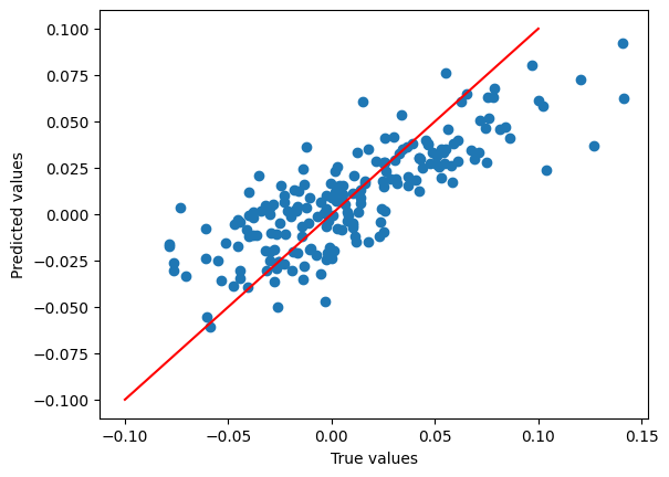
After training, we can now compute some predictions and metrics! We load the regression suite of metrics which can
generate a variety of regression metrics and use the model predictions and the reference values to compute them.
import json

from molflux.metrics import load_suite
import matplotlib.pyplot as plt

preds = model.predict(
    split_featurised_dataset["test"],
    datamodule_config={"predict": {"batch_size": 256}}
)

regression_suite = load_suite("regression")

scores = regression_suite.compute(
    references=split_featurised_dataset["test"]["u0"],
    predictions=preds["ani_model::u0"],
)

print(json.dumps(scores, indent=4))

true_shifted = [x - e for x, e in zip(split_featurised_dataset["test"]["u0"], split_featurised_dataset["test"]["physicsml_total_atomic_energy"])]
pred_shifted = [x - e for x, e in zip(preds["ani_model::u0"], split_featurised_dataset["test"]["physicsml_total_atomic_energy"])]
plt.scatter(
    true_shifted,
    pred_shifted,
)
plt.plot([-0.1, 0.1], [-0.1, 0.1], c='r')
plt.xlabel("True values")
plt.ylabel("Predicted values")
plt.show()
/home/runner/work/physicsml/physicsml/.cache/nox/docs_build-3-11/lib/python3.11/site-packages/lightning/pytorch/trainer/connectors/data_connector.py:424: The 'predict_dataloader' does not have many workers which may be a bottleneck. Consider increasing the value of the `num_workers` argument` to `num_workers=3` in the `DataLoader` to improve performance.
{
    "explained_variance": 0.9999995909535918,
    "max_error": 0.089813232421875,
    "mean_absolute_error": 0.020930099487304687,
    "mean_squared_error": 0.0007172105426434428,
    "root_mean_squared_error": 0.02678078681897608,
    "median_absolute_error": 0.018402099609375,
    "r2": 0.9999995909483964,
    "spearman::correlation": 0.999811745152719,
    "spearman::p_value": 0.0,
    "pearson::correlation": 0.9999997994654302,
    "pearson::p_value": 0.0
}